SC311 Wireless Communications

The objective of this course is to understand how we can transmit a message in-between a transmitter and a receiver spatially separated. Especially, how we can use signal processing operations to adapt (i.e. modulate and demodulate) the message to realize the transmission over wired or wireless channels. This course describes the processes realized at a signal level and can be related to MA331 Information Theory and Channel Coding (which presents the general problem at a higher level).

Slides of the course can be downloaded here. Exercises can be downloaded here. The following of this page corresponds to the labs.

In this labs, we will realize different modulations and demodulations used to transmit and receive analog and digital messages. Spectrum (or power spectral density) will also be determined. Finally, performance, in term of Sinal to Noise Ratio (SNR) or Bit Error Rate (BER) will be estimated in each case.

These labs are based on GNU Radio which is a free software that provides a large number of software blocks to perform most signal processing operations. The blocks are mostly written in C ++. It is possible to use these blocks directly from Python to simulate or create telecommunication systems. In addition, to make it easier to get started, GNU Radio also provides a utility called gnuradio-companion to assemble blocks graphically and to generate the corresponding python script. This subject have been written for GNU Radio, but it can be equivalently realized using Octave, or IT++ library.

Getting Started

• Open a terminal

• Create a working directory in which you will place your scripts.

• Run gnuradio-companion.

This software allows you to use blocks (available in the right column) and to connect them to realize any complex signal processing operations. Resulting program is called a flowgraph in GNU Radio language.

For any flowgraph, there is basically 3 types of blocks: sources (which produce samples and have at least 1 output), sinks (which consume samples and have at least 1 input) and processing block (which have at least 1 input and 1 output). Blocks are simply connected by creating a link in-between an output of a block and an input of another block.

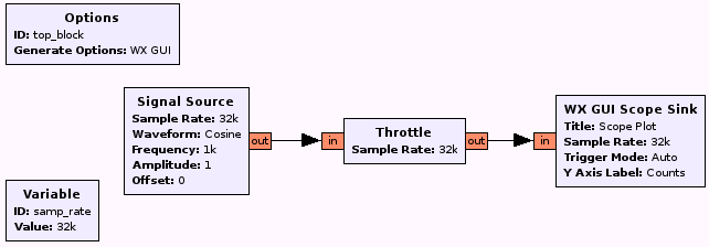
• Create the flowgraph presented in Fig. 1.

Fig. 1: Simple generation and data plotting

The Signal Source block generates an infinity of sinusoidal samples (or other) from the different parameters. These samples are displayed according to the time using the Scope Sink block. Throttle block does not modify the samples but allows to perform a flow control on all the data circulating between the source and the sink. Last, be careful to the color of the input and output of each block since they represent the type of data flowing on the link. The following table presents main data type and associated used by GNU Radio. Also, since Python is strongly typed, colors located at both ends of a wire have to be the same.

Color	Type	Size
Blue	Complex	2 x 64 bits
Orange	Float	64 bits
Green	Int	64/32 bits
Yellow	Short	16 bits
Purple	Char	8 bits

• Save the flowgraph under your directory. This file is saved with a .grc extension.

• Generate the associated Python script associated to your flowgraph using the "blue to red" button. If errors are present, the script is not generated and full listing is present under the no entry sign. When successful, observe the python script named top_block.py in your directory.

• Execute the script by pressing the run button. Equivalently, you can also invoke python top_block.py.

The execution should display an oscilloscope-like widow with the corresponding signal (a cosine function). You can stop the execution by closing the window or by pressing the stop button.

• Check the amplitude and the period of the generated signal.

• Finally, add a Slider block to modify the frequency of the signal in real time (without recompiling the flowgraph) and check the operation on the scope. Save the flowgraph.

Note that the source simply generates samples which are plotted by the sink, however, this source and this sink can produce and consume as much data that your CPU can handle (data are just generated and plotted iteratively as fast as possible). To overcome this issue, the Throttle block is used to process a given number of sample per second, thus lowering the CPU load to few percents. Most of the blocks in GNU Radio do not fixed the rate at which samples are processed: when sufficient number of samples are present at the input, the considered function is called and produces samples at the output which are then available for the other blocks. Usually, this rate is fixed when we work with real devices (for example an audio card can acquire samples at a given frequency e.g. 48 kHz) which fixed the rate for the whole flowgraph. In our example, we do not use any real device so the rate has to be fixed using the Throttle block. Also, for each flowgraph, a single rate has to be used thus if we work with a real device, the Throttle block is not needed anymore and has to be removed.

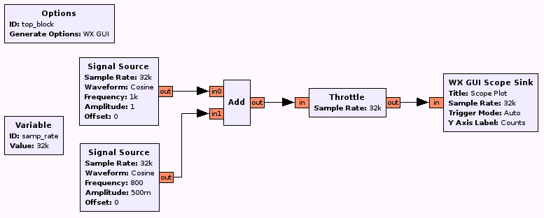
• Create the flowgraph presented in Fig. 2.

Fig. 2: Simple operations on signals

• Add a FFT Sink to observe the signal spectrum. On the graph, the two peaks are very close and seem to be confused. Reduce the frequency sampling to increase the frequency resolution. Explain the phenomenum.

• What is the minimum value of the sampling frequency? Observe the signal (in time and in frequency) for frequencies below this limit.

• Replace the Add block with a multiplier block Mult. Predict the position of the peaks in the output signal. Check your results.

• Add a filter (block Low Pass Filter) to recover the low frequency part of the signal. Check your results in the time and frequency domain. Repeat the manipulation to keep the high frequency part.

The Low Pass Filter (and High Pass Filter) blocks are high-level blocks which realize the design (i.e. determining the coefficients of the filter) as well as the filtering (i.e. the convolution). The filter design can also be done with gr_filter_design to obtain the coefficients. These coefficients can then be used directly by the blocks FIR Filter and IIR Filter.