AC469 Introduction to statistical signal processing

The objective of this lab is to study the effect of the analog to digital conversion. All the exercises can to be done with Matlab or Octave (which is a free software and has the same syntax as Matlab). The preparation part has to be done before the labs. A single lab report has to be done for each group and have to be sent 3 weeks after the end of the last lab .

Introduction

Nowadays, most of the signal processing techniques are done in the digital domain. However, sensors still produce analog signals which need to be converted into the digital domain to benefits from these complex signal processing techniques. Also, this trend is clearly rising since integrated circuit are characterized by constant increase in performance and cost reduction.

The conversion in between the analog domain into the digital domain is done with an Analog to Digital Converter (ADC). This conversion implies 2 different steps:

1. The sampling which consists to transform the continuous time input signal into a sequence of samples.
2. The quantization transforms each sample with a continuous amplitude value to discrete amplitude value and allows a mapping to a binary representation.

The objective of this lab is to characterize the performance of this conversion and to introduce methods which allow to see the trade off and improvements in between to 2 operations.

Preparation

• Discuss about the performance of sampling and quantization on the overall performance. What is the dominant source of error and under which conditions.

Fig. 1: Quantization using rounding method.

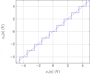
We consider, in the following, that the quantization is done using rounding method. Fig. 1 presents the relation which links the (continuous) input amplitude $x_{i}[n]$ and the (discrete) output values $x_{o}[n]$. The quantization step $q$ is defined as the maximal variation of the input which do not produce a change in the output. Also, note that the function presented in Fig.1 is not a bijection since multiple input $x_{i}[n]$ values has the same output value $x_{o}[n]$. A direct consequence is that it is impossible to reconstruct the continuous input signal form the discrete output signal. Thus this process introduces a quantization error $e[n]$ and is defined as the difference between the continuous value $x_{i}[n]$ and the discrete value $x_{o}[n]$:

$e[n]=x_{o}[n]-x_{i}[n]$

• On Fig. 1, place the quantization step $q$ and quantification error $e[n]$.

Note that, at given sample time $n$, $e[n]$ is a random variable.

• Give the maximum value and minimum value of $e[n]$ and determine its associated probability density function $p_{e}(x)$.

• Determine the mean $m_{e}$ of $e[n]$ defined as:

$m_{e}=E\left[e[n]\right]=\int _{-\infty }^{+\infty }xp_{e}(x)\mathrm {d} x$

• Determine the variance of $e[n]$ defined as:

${\text{Var}}(e)=E\left[(e[n]-m_{e})^{2}\right]=\int _{-\infty }^{+\infty }x^{2}p_{e}(x)\mathrm {d} x$

• From these results, determine the power associated to the quantization error.

We suppose now that we want to apply the quantification process for the signal $x_{i}[n]=A\cos 2\pi f_{0}t$ over $N$ bits using rounding with a full scale of $2A$.

• Determine the expression of the Signal to Noise Ratio (SNR) in decibel as a function of $N$. What is the expected improvement in SNR when we increase $N$ by one?

Classical Quantization

Start Matlab or Octave, these 2 software accept commands which can be directly entered at the prompt, or placed inside a script (an external file with an extension .m) in the working directory. Function can also be placed inside a file (whose name is identical to the function and with an extension .m, see below for an example). For each command, detailed prototype is described in the (online) manual.

• Generate a vector of 10 samples with a normal distribution using the command:

x = randn(1,10)

• Matlab (and Octave) makes a difference in between row (or line) vector and column vector: inverse 1 and 10 and observe the result. Add a ; at the end of the previous command and observe the result. Value at a given index n can be accessed by x(n). Note that Matlab is "1-based" which means that the first element of a vector starts a 1 (and not 0). Note that last element can be accessed by end

• Plot your vector using the following commands (type the commands one at a time):

plot(x);
stem(x);
hist(x);

• Generate a new vector with 1000 samples. Determine the mean value, the minimum and maximum values, the standard deviation and the variance of your vector.

• Generate another vector of mean $\mu =3$ and variance $\sigma ^{2}=2$.

• Write a new function to realize the quantization over N bits over a full scale of 2A. Check your function by considering the signal xi = linspace(-A, A, 1000);. Be careful to implement a saturation so that the number of possible output is equal to $2^{N}$.

• Run a simulation to compare the experimental SNR to the theoretical SNR obtained in the preparation part from $N$ to 1 to 8.

Quantization with oversampling

• Generate a signal $x_{i}[n]$ composed of the sum of 3 harmonic functions sampled at a frequency of $f_{s1}=44.1$ kHz and $f_{s2}=4f_{s1}$. Each function parameter is available in the following array:

Frequency (Hz)	Amplitude (V)	Phase (deg)
440	1	0
546	0.3	0
999	0.7	0

In the following, we note $x_{1}[n]$ the signal sampled at $f_{s1}$ and $x_{2}[n]$ the signal sampled at $f_{s2}$.

• Plot the different curves in time and frequency domain. Discuss about the resolution in each domain.

Oversampling

The objective of this part is to characterize the performance degradation which is classically achieved when a signal is oversampled. For this, a new version of $x_{2}'[n]$ should be constructed from $x_{1}[n]$ and compared with $x_{2}[n]$.

• From a theoretical point of view, what is the maximum SNR which can be achieved by comparing $x_{2}[n]$ and $x_{2}'[n]$.

• From x1, generate the interpolated vector x2p using the interp1() function. Modify the interpolation method, plot the results and characterize the SNR in each case.

Digital filter design

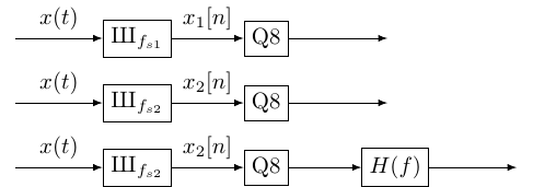
We consider the three different systems presented in Fig. 2. The first one corresponds to quantization over 8 bits at a frequency $f_{s1}$, the second one is identical except that the sampling frequency is $f_{s2}$. The last one is different since a digital filter have been added after the quantization.

Fig. 2: Different quantization types.

• Simulate the first system by considering that the input signal is $x_{i}[n]$. After the quantification, determine the SNR compared $x_{i}[n]$ sampled at $f_{s1}$.

• Simulate the second system by considering that the input signal is $x_{i}[n]$. After the quantification, determine the SNR compared $x_{i}[n]$ sampled at $f_{s2}$.

• For the third system, establish first the characteristics of the digital filter. Then use the following function to generate the impulse response $h[n]$.

function h=fir(N,f0)
% FIR Filter
% N  = impulse response length
% f0 = normalized cutoff frequency

f = linspace(-0.5,0.5,100);
ham = 0.46+0.54*cos(2*pi*f); %window function (hamming)
h = sin(2*pi*f*N*f0)./(pi*f*N); %sinc function
h = h.*ham;

• From the impulse response, check in the frequency domain that the magnitude of the transfert function satisfy your design.

• Implement the filter by realizing the convolution in between $x_{2}[n]$ and $h[n]$

• Finally compute the SNR compared $x_{2}[n]$ sampled at $f_{s2}$ (be careful that a convolution introduce a delay which need to be compensated to correctly estimate the SNR value).

Noise Shaping

In the previous section, we have seen that performance can be increased by increasing the sampling frequency and using a (carefully designed) digital filter. In this section, we will see that the performance can also be increased by modifying the power spectral density of the quantization noise. We consider the system presented in Fig. 3. Note that after $H(f)$, digital signal is usually down sampled to a lower frequency, as we have seen earlier, this operation do not modify the signal to noise ratio.

Fig. 3: Noise shaping.

Theoretical study

• Express $z[n]$ as a function of $x[n]$ and $e[n]$.

This system has the propertie to process the signal and the noise differently using 2 different transfer functions.

• Set $e[n]=0$ and express the transfer function in between the input $x[n]$ and the output $z[n]$. Conclude on the behavior of this filter.

• Set $x[n]=0$ and express the transfer function in between the input $e[n]$ and the output $z[n]$. Conclude on the behavior of this filter (you can determine the magnitude of the transfer function).

Implementation and simulation

• Implement this system on Matlab or Octave. Observe the different signals. Plot the PSD of $e[n]$.

• Determine the improvement of this technique compared to the previous ones.

Conclusion

All the techniques presented in this lab are implemented and used in Delta Sigma ADC to increase the performance of the conversion where simple 1 bit ADC can produce more than 18 effective bits (and an oversampling ration of 64). Due to the limited speed of conversion, all these technique are only applied on low bandwidth signals (mostly audio).